December 6th 2017 - Tejpal Virdi
Introduction
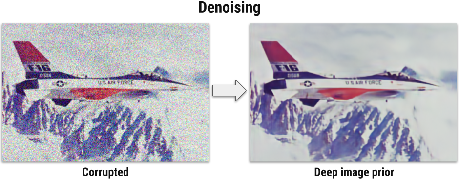
Recently, Ulyanov et. al introduced a paper titled “Deep Image Prior,” describing how a great deal of image information can be captured simply by the structure of a convolutional neural network. They use this inherent nature of ConvNets to perform various image restoration problems, where the “prior” is needed to restore the lost information. Rather than learning from a set of images, this technique demonstrates that the CNN itself encapsulates the image. This is notable since most previous attempts to solving problems in single-image super-resolution, denoising, and inpainting all required the use of large datasets or complex algorithms. In this post, we show how this methodology can be used to enhance the quality of noisy audio samples.
Deep Image Prior
As briefly mentioned in the introduction, Deep Image Prior utilizes the fact that the generator network itself has the answer to the restoration problem. Thus, the solution set is in the network’s parameters rather than the general image space. This motivates the development of new deep learning architectures that are domain-fitted for improved accuracy. Here are some results from the original paper:
Audio
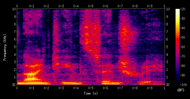
Audio is commonly generated as a WAV file, which contains the pure signal of the audio. However, since that is extremely dense and large, we must convert it into a representation that would reduce computational expense. Specifically, audio can be visually represented in terms of a spectrogram, which shows the distribution of frequency over time. As an image, it is not lower in dimensionality and we can use a plain old ConvNet to learn from it. (Note: Recurrent Neural Network architectures are more often used with audio since previous states/history tends to have an effect on the current state )
Methods and Results
We employ a DCGAN trained on one degraded image. Throughout the training, we sample its outputs. Here are the network’s outputs over ~2000 iterations:
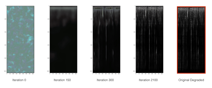
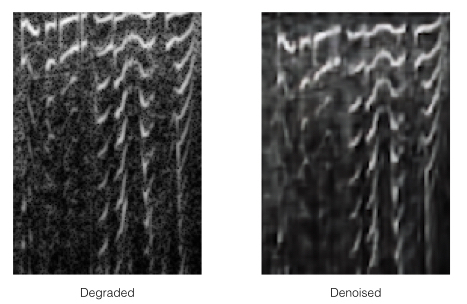
As seen in the figure, the network is initialized with random weights and learns the different features of the degraded image. The network, however, does not learn the noise of the spectrogram so the generated images are of higher quality than the input degraded image, as seen below:
Implementation available here