November 3rd 2017 - Tejpal Virdi
In our previous blog post we discussed the effectiveness of Neural Networks for image classification tasks comparable to humans. However, how good are neural networks at being creative? Here we explore the Generative Adversarial Network: the most effective generative model used today.
The Generative Adversarial Network is made up of two networks. One network is known as the discriminator and the other is the generator. The main idea behind the GAN is to have these two networks compete with each other. The discriminator is tasked to identify between real and fake samples of a certain class of image, while the generator tries to produce more realistic images that fool the discriminator. The two networks are trained simultaneously, and the idea is that the competition will drive them to produce synthetic data that is indistinguishable from fake data.

Discriminator
The discriminator is essentially a standard CNN like from our previous blog post. It is a binary classifier, meaning that there is only one output node representing a value from 0-1, which indicates the probability of it being real or fake. A probability of 0.5 will mean that the discriminator cannot tell if the input was real or fake. We can respectively subtract this value from 1 to get the corresponding opposite probability. The discriminator uses the cross entropy loss formula denoted as:
Generator
The generator is a deconvolutional network. Just as the name suggests, it essentially works in a reverse manner to the standard convolutional neural network. Instead of reducing an image into a lower dimensionality for feature extraction, as did the CNN, the generator takes in a random noise vector as up-samples it.
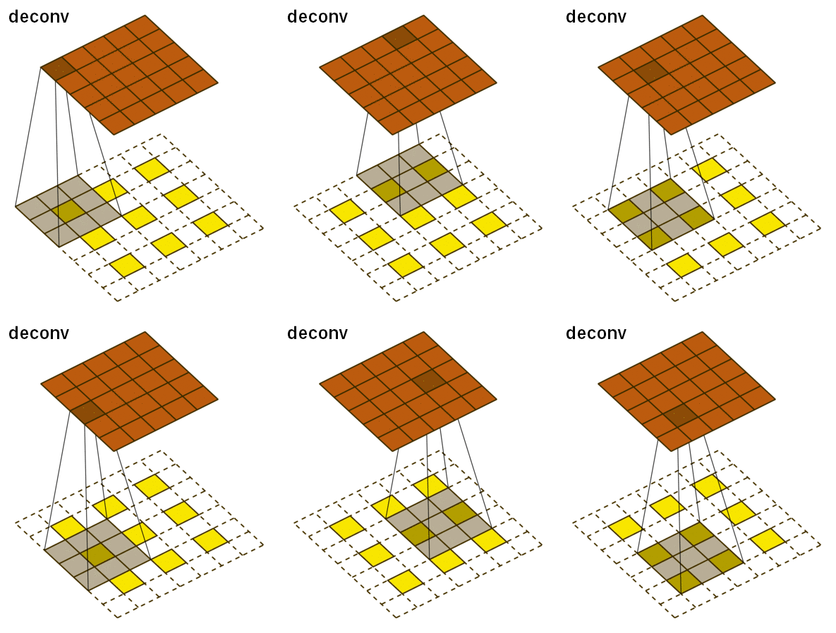
The deconvolutional network has the three main layers: deconvolution, unpooling, and ReLU. The deconvolutional layer starts off with a feature map and for each pixel value, it maps it to a square kernel, upsampling the image. This is done for each feature map and can be thought of as a matrix multiplication between the transpose of the whole filter matrix and the input. This is what it looks like:

For unpooling, we must revert the pooling operation by going from a single pixel to a 2x2 array of pixels. However, it is impossible to do this accurately based off guessing. Instead, our network uses switch variables to memorize the pooling operations from the convolutional layer to accurately reconstruct the image.
The last layer is simply applying the ReLU to add a nonlinearity. The ReLU is simply an activation function and does not change the resolution of the image. See the blog post on CNNs for more information on ReLUs.
Adversarial Training
The fascinating part of GANs is its use of adversarial training. Meaning, the generator and discriminator networks act as adversaries in terms of their loss functions. This is based off of the minimax game in Game Theory.
The distributions, p and q, are given by our example training data and the generator, where the training data refers to real, and the generated images refer to fake. Because we only have two classes, the loss function can be simplified to the binary cross entropy function:
X1 represents one input data point and y1 represents our label (not the entire dataset). However, because we feed the discriminator exactly half real and half fake data, we need to encode this probability, the loss function therefore becomes:
We first train the discriminator with training data (we used MNIST). The input is passed through a series of convolutional layers (downsampling the image to extract features) and ReLUs, ending with a Sigmoid activation. The loss is computed using the original MNIST labels. Next, the generator model is called on a random noise and the output of that is run through the discriminator, computing the loss (The output is compared with a set of fake labels). We then do backprop on the discriminator, given that it has now analyzed both real and fake images.
Next, we must train the generator. We have it produce images given random input and put those synthetic images through the discriminator, giving us a loss. We use this loss to perform backprop on the generator model and repeat this whole process for a given number of epochs. The code for this process is broken down below