October 29th 2017 - Tejpal Virdi
Over the last weekend, we committed ourselves to learning exactly how a neural network (NNs) works. This intro blog post will teach you everything you need to get a straightforward neural net running. To start off, here is what the architecture of a simple 2-layer NN looks like:
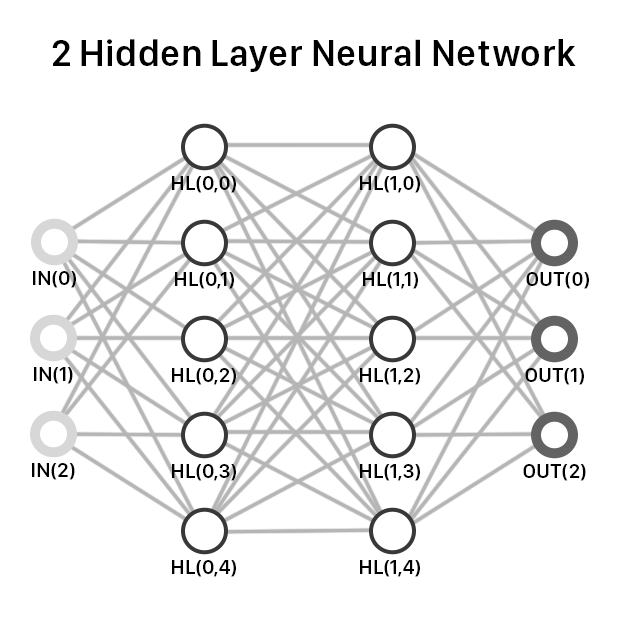
The learning process in neural nets has two parts: A forward pass and a backward pass. As seen in the diagram above, the inputs go through each layer in the forward pass until reaching the output layer. From there, each output node passes information back through the network to make adjustments for the next forward pass.
Forward Pass
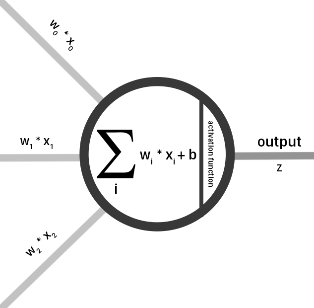
The first layer of a neural network is the input layer and each input node in the input layer is connected to every hidden node (fully-connected). For each connection between nodes in the input and hidden layers, there is a individual weight matrix that the input is multiplied by. The output of this multiplication is summed across all other connections to the same node. This can be simply expressed as neat matrix multiplications between the input and weights matrices. For example, if our input matrix is of size 1x3, and our weights matrix would be of size 3x5, we would have 15 individual connections.
The next step of the forward pass is applying the sigmoid function on the values obtained from the multiplication between the input and first weights matrices. The sigmoid function is:
and maps the input into a value from 0 to 1, also adding a nonlinearity to the model. The sigmoid function is what ultimately allows us to curve fit to our desired function.
We have now finished the pass from input times weights times sigmoid. If you are familiar with Biology, this can be visualized as a neuron. The dendrites are the input and weights, the cell body is the multiiplication and activation, and the output axon is the sum of the multiplications.
We then repeat how we passed the data through the input nodes to HL1 (hidden layer 1) when going from HL1 to Hl2. We multiply the hidden layer 1 values with a second weights matrix and apply the sigmoid function. To go from the HL2 to the output layer, we repeat the process again.
Backpropagation
Once we have our output, we need to evaluate how well the weights did in the forward pass. Using the training data as labels, we can calculate the loss using a formula known as mean squared error:
Using this loss and basic calculus, we can approximate how we need to adjust our weights to minimize the loss. Our goal is to find how much the loss will change from a change in the weights, or:
This term expresses how much the loss increases or decreases when we make a small change to a weight. By following how we evaluated our loss and applying the chain rule, we can calculate this term. Going backwards, the most final function we apply to get our error is MSE. Using the power rule we can calculate the derivative of this function:
Next, we must calculate the derivative of step before we calculate the output, which was the sigmoid function:
Finally, we calculate how the weight influenced the output (pre-sigmoid):
Now that we have seperated calculated the derivative of each “chained” function, we can finally calculate the derivative between the loss and weight 0:
To update each individual weight, we apply the formula appropiately and calculate the new weight through:
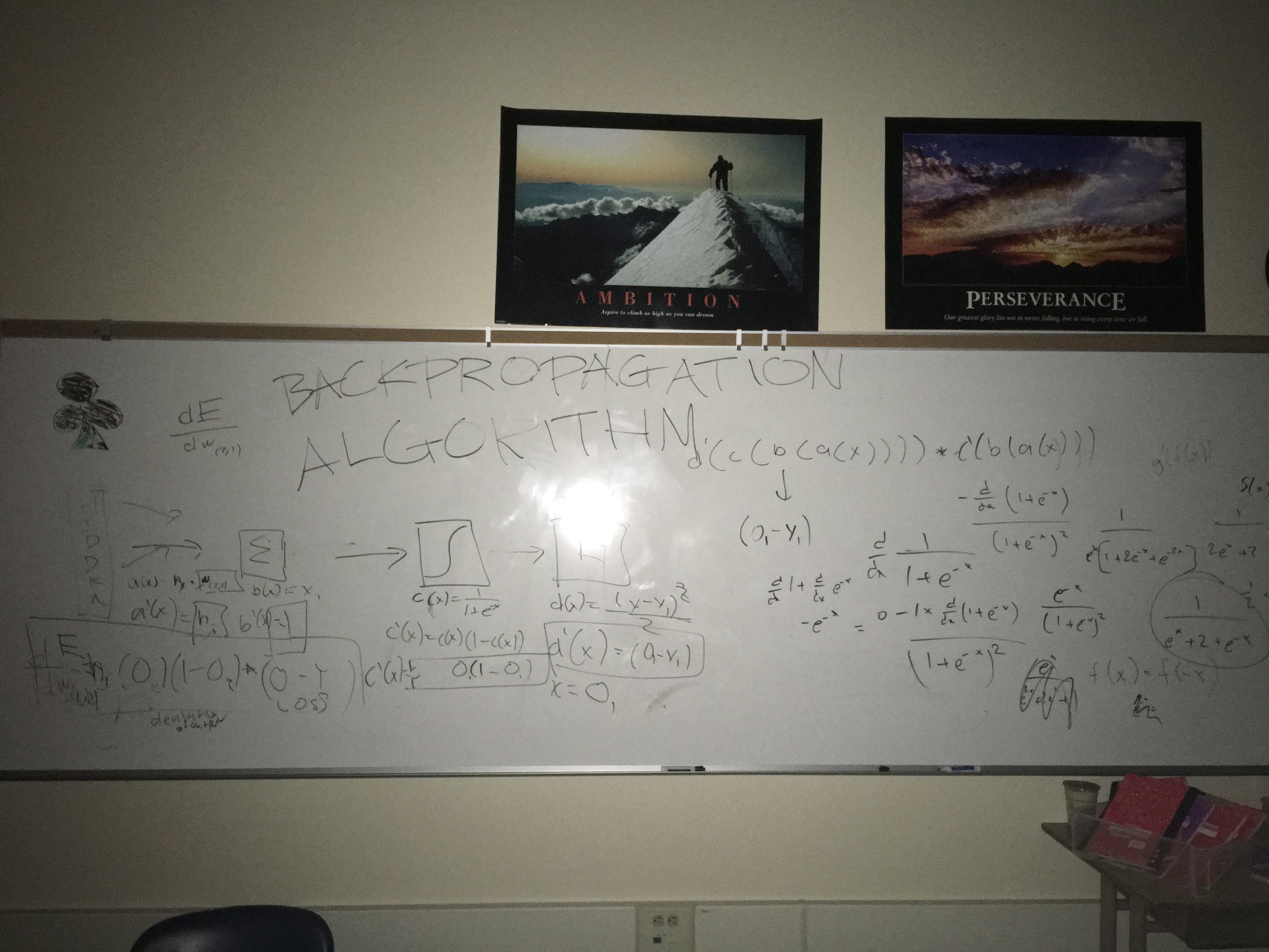
We had some extra time so we wrote it out…(it was 3am at a hackathon in our math classroom)