October 29th 2017 - Tejpal Virdi
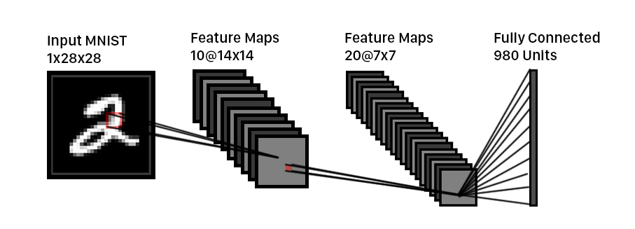
Convolutional Neural Networks (CNNs) are a certain type of Neural Network that excel at image recognition and classification. They are used to analyze an image through the extraction of relevant features and have special characteristics that allow it to perform better on 3D and 2D volumes of data. Through a series of layers, the CNN extracts relevant features from the input image. The four main layers are known as convolutional layers, ReLUs, pooling layers, and fully-connected layers. Just as how an artificial neural network can have multiple hidden layers, a deep CNN may repeat these layers multiple times.
If you are new to neural networks in general, we recommend that you visit our introductory blog post first.
Convolutional Layer
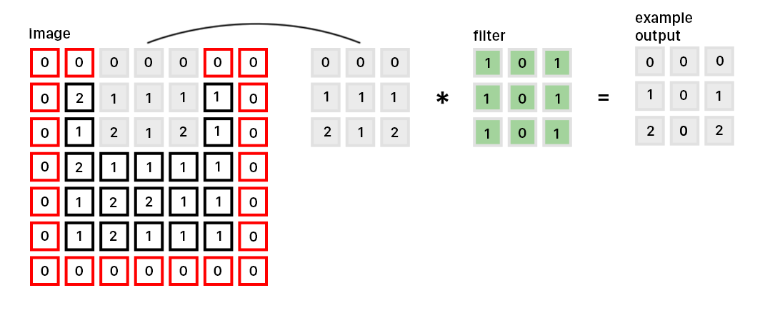
The Convolutional Layer is the meat of the whole process. Similar to the neural network, the convolution layer has a set of learnable weights, called filters. The filter is usually of a size smaller than 10x10 pixels and slides across the image, computing the dot product between the input pixels and filter. The resulting matrix is known as an activation map and can be stacked spatially to produce the output volume.
Here are some important terms to know: the size of the filter is often known as the kernel size, stride refers to how many units the filter moves every iteration of the convolution, and padding refers to the zeros you add around the image so the filter can be applied onto pixels nearing the edges of the image.
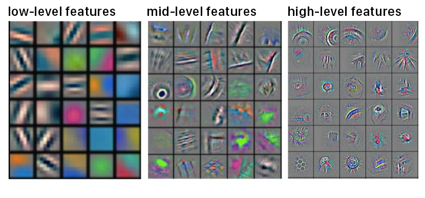
For image recognition, the filters learned usually represent lower to higher spatial features. For example, filters in the first convolution might represent edges or corners. Through the combination of these lower level filters, filters in later convolutions are able to take this information and look for higher level features such as faces.
ReLU
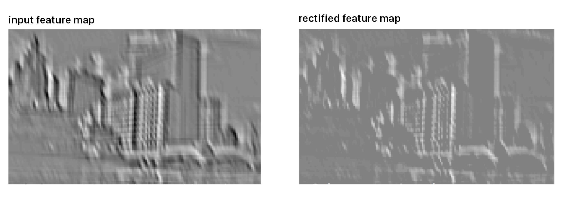
Rectified Linear Units (ReLUs) serve as activation functions, and are simply defined as:
The simplicity of this function allows for improved training speed, in both the forward and backward passes. Observe that computing the gradient of the function simply returns a 0 or 1, only dependent on sign of x. In comparison, logistic and hyperbolic activation functions, such as the sigmoid function, are prone to the vanishing gradient problem. The vanishing gradient problem is based on the gradients having an infinitesimal effect on the output. A local minimum of the loss function is found and the small changes of the gradients prevents the model from learning. However, ReLUs are not subject to this since their derivatives are simply 0 or 1.
Pooling Layer
To understand an image, the CNN must downsample it to include only relevant information. Pooling layers are used to reduce the spatial size, thus reducing the total number of parameters of the model. This lowers computation time and prevents overfitting since the output of the pooling layer is a more general representation of the input.
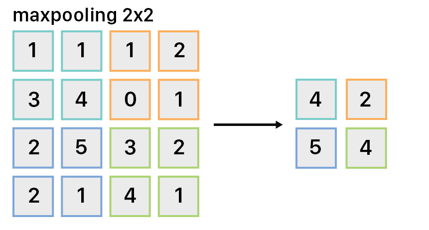
A simple type of pooling is max pooling, which applies a filter of size, let’s say, 2x2 across the image. For every 2x2 set of pixels on the input, it will only keep the maximum pixel value and remove the rest, thus downsampling the image by 4x in our example. Note: this filter preserves depth to keep an accurate spatial representation of the input.
Fully-Connected Layer
Fully-connected layers are used at the end of the model as a nonlinear transformation, by a simple matrix multiplication, to go back from activation maps to relevant high-dimensional data. The channels of information are flattened, and their spatial representation is lost. It is important to note that a fully-connected layer is the same thing as performing a convolutional layer with the kernel size as the size of the image.
Forward Pass
 The forward pass simply involves running the input image through each of the filters, pooling layers, and ReLU’s.
Backpropagation
In the case of CNNs, backpropagation is used to make adjustments to the filters in order to get a lower loss. It is calculated similarly to the artificial neural network, however it accounts for the addition of filters. (see blog post on simple neural networks, more math explained there)
Current Architectures
Within the last few years, many new CNN architectures have come out. It’s helpful to be familiar with them since you will most likely encounter them in practice. We will briefly look at AlexNet, VGGNet, and ResNet.
AlexNet became popular after its submission to the annual ImageNet ILSVRC competition in 2012. It’s key features are its significant depth as well as its use of stacked convolutional layers without pooling after each one.
The VGGNet showcased the importance of depth in a CNN architecture. The model contained 16 convolutional and fully-connected layers with convolutions of size 3x3 and 2x2 for pooling. However, due to the depth and large number of fully-connected layers, the net ended up having over 140 million parameters, making it computationally expensive in terms of both memory and time.
The ResNet is a residual network that removes many of the drawbacks of the VGGNet, being extremely efficient through the use of skip connections, absence of fully-connected layers, and significant use of batch normalization. A skip architecture is where the network gives the output of a layer to the next layer as well as the one after it, thus skipping to the next connection. Batch normalization is a used to normalize the distribution of the input across the batch. It scales and shifts this distribution, allowing for a more stable training process. This also allows for a higher learning late without getting stuck in a local minimum of the loss function.