05 Oct 2017

October 5th 2017 - Tejpal Virdi

Introduction

This blog post demonstrates the process of analyzing a set of images with the goal of identifying an average face, prominent face, eigenface, and recognition system. The process utilizes the mathematical concepts of matrices, eigenvalues, and eigenfaces (formally known as eigenvectors) with the goal of reducing a high-dimensional space from a large data set of pixel values. The eigenfaces (eigenvectors) compose a face space (eigenspace) in which a variance is identifiable and can be operated on through the process of Principal Component Analysis. Each image is read by its pixel’s grayscale values from 0-255. The process of face recognition through eigenfaces differs from other face recognition processes since features are not visualized in 3D space and distinctive features (nose, ears, eyes, etc.) are not identified.

Eigenfaces

The first step when dealing with face images is to represent each image Ik as a column vector of grayscale values for each pixel. This process can be thought of as transposing each of the N rows of N pixels into a $N^{2}$ x 1 column vector and essentially visualizing an image as a point in N2 dimensions. An average face can be found by summing the column vectors of each image and dividing entries by the scalar M (# of images). Prominent parts of each face are found by subtracting the average face from each face in the set of images, denoted as Φi=Γi−Ψ. The prominent faces are put in the matrix A where $A * A_{T}$ represents the covariance matrix. However, this matrix is high-dimensional ($N^{2}$ x $N^{2}$) and must be reduced by taking the inner product $A_{T} * A$ (M x M dimensional). The process of obtaining the covariance matrix is what is known as Principal Component Analysis (PCA). Although the result is a simple matrix multiplication, the process of PCA is quite complex and will be discussed in the upcoming paragraph. Once the covariance matrix is obtained, the M eigenvectors and eigenvalues can be computed. These eigenvectors can be rendered on the screen to appear as eigenfaces. The process of face recognition and reconstruction utilizes the concept of weights to express an input image as a sum of eigenfaces.

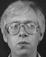
The first step is to find a set of images you can use as a training set. I would recommend using the AT&T Cambridge Face Set, or the Yale Face Database. We used the faces available online of the Gunn Math Faculty. We will refer to the size of this image set as M. Each image will then be referred to as of ${I}\ or \ I_{1}, I_{2}, I_{3} \ ... \ I_{M}$

$$I_{k} = \begin{bmatrix} p_{1} &p_{2} & \cdots &p_{a} \\ p_{a+1}& p_{a+2} & \cdots&p_{2a}\\ \vdots & \vdots & \ddots & \vdots \\ p_{3a+1}& p_{3a+2}& \cdots & p_{4a} \end{bmatrix}$$

To make our recognition more effective we must set the standards for our images.

1. The images must be face aligned.

2. Must be of the same dimensions N x N

3. Must all be of grayscale values from 0 - 255 (recommended)

We can represent each image as a N x N matrix where each element corresponds to the gray scale value of a pixel.

Once we have that our next step is to convert each image into a single point in a $N^{2}$ dimensional space. We do this by transposing each row one by one and appending each row below one another to create a $N^{2}$ x 1 column vector. We repeat this for every image in the set. By systematically appending each row of the I matrix we can get a vector that looks something like this:

$$\Gamma = \begin{bmatrix} p_{1}\\ p_{2} \\ p_{3} \\ \vdots \\ p_{n} \end{bmatrix}$$

Because we are looking for the most distinguishing parts of each face we compute the average face. This can be done using $\Psi = \frac{1}{M} \sum_{i=1}^{M} \Gamma_k$. If we now subtract each face $\Gamma_k$ from the average face we are left with the most prominent parts of each input image. $\Phi_i = \Gamma_i - \Psi$ , $\Phi_i$ is the prominent image of each face. This is intuitive as we are taking each face and subtracting the qualities that are common between the face set.

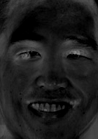
As you can see in figure above, the prominent face only leaves the most important characteristics of a face that changes from person to person. You can see how the areas around the eyes and teeth are much lighter than their surroundings.

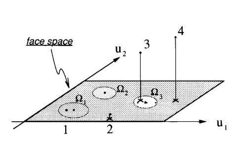
Now we have a set of points in a high dimensional space that represent each face most prominent features. This is now where we apply principle component analysis or PCA to find the most important eigenvectors that represent the distribution of our data without losing important information.

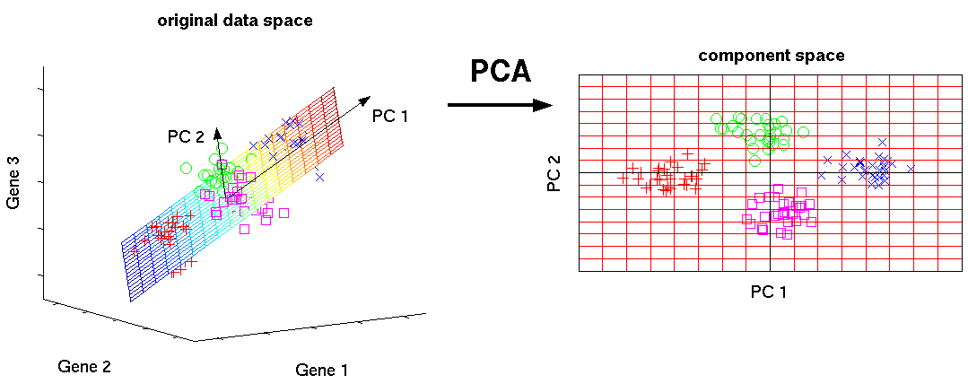
As you can see in figure above, although initially the points were described in a three dimensional space, because most of the points are along a two dimensional plane we were able to find two orthogonal vectors otherwise known as principle components or eigenvectors to describe the plane. If you define these components as the axis of a new space, you are able to make a subspace with reduced dimensions. This idea can be applied to our high dimensional data set and reduce the size of our data from $N^{2} \rightarrow M$dimensions. The efficiency gained by reducing the dimensions outweighs the data loss.

We use what is called a covariance matrix (Matrix C) which can be computed through $C = \frac{1}{M} \sum_{i=1}^{M} \Phi_i \Phi_i^T$. This summation produces $\left[ \Phi_1^2 + \Phi_2^2 + ... \Phi_M^2 \right]$ which is the definition of variance.

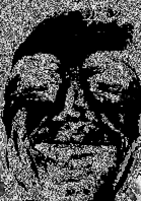
Computing all the eigenvectors of a $N^{2}$ space can be very daunting for a computer, fortunately through PCA we know that we can use C, a M x M matrix to help us find these vectors much more quickly. By directly finding the eigenvectors of C we can use a formula to compute the respective eigenvectors of the data set. This can be done through: $u_i = A v_i$ where u represents the eigenface, A is the set of column vectors and v is the corresponding eigenvector of matrix C. This is how you find the eigenfaces. We can render these vectors by scaling them to 255. These eigenvectors are often slightly recognizable as faces, hence the name eigenfaces. Here is an example:

Reconstruction & Recognition

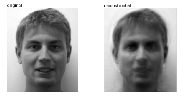
Now that we have found all the eigenfaces we can essentially express every face in the high dimensional space as a sum of these eigenfaces. Therefore in theory we should be able to reconstruct every face fairly well although we will lose some quality due to our dimensionality reduction during PCA.

$$\Omega = U^T (\Gamma - \Psi) = \begin{bmatrix} \omega_1 \\ \omega_2 \\ \vdots \\ \omega_R \end{bmatrix}_{M \times 1}$$

We can figure out how to reconstruct the face using this formula which will return the weights of each eigenvector used. By using the weights and adding those eigenfaces we can reconstruct a face. In figure 6 above we can see how eigenfaces were used to reconstruct the original image on the left. The reconstructed image is slightly blurry due to PCA but the most important information is still intact.

Then by looking at their weights and comparing those weights to the weights in the training faces, we can identify if in a certain input face was in the training set. We can systematically due to this by setting a certain threshold and calculating the euclidean distance. $\epsilon = \left\| \Phi - \Phi_f \right\|$. If this distance is lower than the threshold we set we have successfully identified the face.

Conclusion

Although eigenfaces are a successful method of facial recognition, it is not the best out there. Some of the drawbacks of eigenfaces are how the set of images must be taken under the same scenario. For example input images where the lighting is different could significantly affect the eigenvectors this could result in the system starting to identifying faces from their light levels instead of their faces. A more effective form of facial recognition would be to treat the face as a three dimensional object instead of two dimensional like we did with an image. This allows would allow us to recognize an image from multiple angles and would not be affected from lighting as well as light can be manipulated in the three dimensional world.

Overall, facial recognition has proved to be a very useful tool in many areas of life. For example facial recognition can be used for security, social media, or targeted advertising. As we rely more and more on sensory technology to help us interact with our surroundings, it is important for us to create better facial recognition systems.

Java Code